Artificial Neural Networks and coastal applications
Artificial Neural Networks (ANN)s are a powerful technique for analyzing large data sets representing observations of natural phenomena and possible influencing factors. It can identify and quantify hidden patterns and correlations without prior information about the dynamics of the underlying causes. Once these patterns and correlations are established, the neural network can be used as a prediction tool for unobserved situations. An important restriction is that predictions can only be made for phenomena that fall within the range of the observed situations. ANNs can also be used to investigate the sensitivity of the output to input data of various possible causative factors and thus provide information about the factors that most strongly influence the targeted phenomenon. It is also possible to estimate the uncertainty margins of predictions by training the neural network on different subsets of the observation data. The practical importance of neural networks has been strongly stimulated during the past decade by the availability of large data sets (for example from remote sensing and continuous in situ observations) and data repositories and by the sharp increase in available computing power.
Contents
Background
Hodgkin and Huxley (1952)[1] performed pioneering experimental studies on current propagation along the giant axon of a squid, consequently developing the first detailed mathematical model of neuron dynamics. The model is the first to include multiple ion channels and synaptic processes, as well as realistic neural geometry (Gerstner and Kistler, 2002[2]). Following this work, several researchers started to study interconnected neurons as an information processing system, developing the theory of artificial neural networks. The term 'perceptron' was introduced by Rosenblatt (1961)[3] during this time to refer to an artificial neuron, rather than a natural one. However, according to Kingston (2003)[4], the origin of artificial neurons may be traced back to McCulloch and Pitts (1943)[5]. In the following the term neuron is also used for artificial neuron. In other publications the term 'node' is sometimes used for an artificial neuron.
Neural feedforward network design
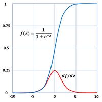
The propagation of a current along the main body of a cell in natural neural network and subsequent release of ions in the synapses is modeled in an artificial network by a feedforward mechanism between artificial neurons. A natural neuron transmits ions to other connected neurons when it receives an excitation impulse above a certain level. In artificial neural networks the release of ions is simulated by an activation function whose output depends on the received inputs. In small networks the activation function is often modeled by a sigmoidal function [math]f(z)[/math], for example the logistic function (see Fig. 1)
[math]f(z)=\Large\frac{1}{1+e^{-z}}\normalsize . \qquad (1)[/math]
The number of inputs and the form of the activation function may vary, and the precise form of the output may vary accordingly.
The aim of an artificial network is to predict the value [math]Y[/math] of a particular target property knowing the values [math]X_i, \; i=1, .., n[/math] of a set of [math]n[/math] related or influencing factors. An artificial neural network therefore consists of the following elements:
- A set of input data [math]X_i, \; i=1, .., n[/math] provided by the user, each of the input data corresponding to a factor that the output is assumed to depend on or to be related to;
- A user-defined configuration of one or more interconnected layers of neurons (so-called 'hidden layers') that convert the input they receive into an output according to a user-defined algorithm based on weight parameters;
- The output [math]\hat{Y}[/math], the value of the targeted property which is generated by the neural network based on weight parameter values determined by previous adjustment to a set of training data.
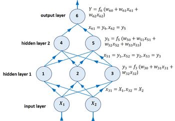
The first hidden layer receives input from the user-provided data; the next hidden layers get input from other hidden layers. In a typical feedforward network, all neurons of subsequent layers receive all input from all neurons in the preceding layer, see Fig. 2. The output [math]y_k[/math] of a neuron [math]k[/math] is given by
[math]y_k = f_k(z_k), \quad z_k = \sum_{i=0}^{n_k} w_{ki} x_{ki} , \qquad (2)[/math]
where [math]f_k[/math] is the activation function of neuron [math]k[/math], [math]n_k[/math] is the number of inputs [math]x_{ki}, \; i=1, .., n_k[/math] received by neuron [math]k[/math]. The neuron has weight parameters [math]w_{ki}, \; 1=0, ..,n_k[/math]. By convention [math]x_{k0}=1[/math] and [math]w_{k0}[/math] is the so-called bias. The neurons in the first layer receive the set of given inputs [math]X_i, \; i=1, ..n[/math]. Connections with a positive weight are called excitatory, the ones with a negative weight are called inhibitory. The activation function transforms the sum nonlinearly into a number which is transmitted as input to the next layer. This feature of the activation function is essential for the capability of the neural network to simulate nonlinear processes.
Network training
Gradient descent procedure and backpropagation
The performance of a neural network depends on the values of the [math]n_k[/math] weight parameters [math]w_{ki}, \; i=0, .., n_k, \; k=1, .., K[/math] for each of the [math]K[/math] neurons. For a deep network with many inputs and many layers the number of weight parameters can be very large. Network training consists of finding values of the weight parameters from training data. Training data [math]X_{ji}[/math] consist of a set of training conditions for which the outcome [math]Y_j[/math] is known. The first index [math]j=1, .., m[/math] indicates one of the [math]m[/math] training examples and the second index [math]i=1, .., n[/math] one of the [math]n[/math] corresponding input parameters. The training process consists of the iterative updating of the weight parameters in order to stepwise reduce the difference between the network output [math]\hat{Y_j}[/math] and the known outcome [math]Y_j[/math] for all [math]j=1, ..,m[/math], which we call the error [math]E[/math]. The error is usually defined as the sum over all training examples of the squared deviations between network output and training data (as in maximum likelihood estimation from a statistician point of view),
[math]E = ½ \sum_{j=1}^m (Y_j - \hat{Y_j})^2 . \qquad (3)[/math]
The error is smallest when any change in one of the weight parameters [math]w_{ki}[/math] increases the error, implying that at minimum all partial derivatives [math]\partial E / \partial w_{ki}[/math] are zero. Convergence to the minimum is achieved by updating the weights [math]w_{ki}[/math] such that each update produces the greatest error decrease,
[math]w^{t+1}_{ki} = w^t_{ki} - \eta \; \partial E / \partial w^t_{ki} \; , \qquad (4)[/math]
where [math]w^t_{ki}[/math] is the value of the weight parameter value [math]w_{ki}[/math] at iteration step [math]t[/math], [math] \; \partial E / \partial w^t_{ki}[/math] the partial derivative of the error with respect to the weight [math]w_{ki}[/math] at iteration step [math]t[/math] and [math]\eta[/math] is a user-defined hyperparameter that determines the magnitude of the steps towards the minimum. Equation (4) implies that the weight parameters are updated in proportion to their contribution to the error gradient; this minimization procedure is called 'gradient descent'. For a particular neuron the update is (dropping the index [math]k[/math] and using the expressions (1-4))
[math]w^{t+1}_i = w^t_i + \eta \sum_{j=1}^m (y_j - \hat{y_j}) \large\frac{\partial \hat{y_j}}{\partial w_i}\normalsize = w^t_i + \eta \sum_{j=1}^m (y_j - \hat{y_j}) \large\frac{\partial f}{\partial z}\normalsize \large\frac{\partial z}{\partial w_i}\normalsize = w^t_i + \eta \sum_{j=1}^m (y_j - \hat{y_j}) \hat{y_j} (1 - \hat{y_j}) x_{ij} , \qquad (5)[/math]
where [math] ½ \sum_{j=1}^m (y_j - \hat{y_j})^2[/math] is the contribution of this neuron to the total error [math]E[/math]. A special procedure is needed to determine the contribution of each neuron to the error [math]E[/math]. This procedure consists in propagating the error back through the network and is called backpropagation. It is an essential feature for training feedforward neural networks.
Vanishing gradient issue
The backpropagation procedure involves products of the gradients of the activation functions for successive layers. Therefore some activation functions are less suitable than others. A step function to simulate a neuron excitation threshold is unpractical because the derivative is zero or not defined. The logistic function is also less suitable because the gradient is generally much smaller than 1 (Fig. 1), implying that the error is not well propagated back through large networks. Therefore other more suitable activation functions are generally used, in particular the so-called rectified linear unit (ReLU) function,
[math]f(z)= max[0, z] . \qquad (6)[/math].
Multiple minima issue
The sum of squared deviations is a nonlinear function in the (huge) multidimensional space of all weight parameters (including biases). Through the backpropagation procedure the steepest gradient towards the minimum error in the space of weight parameters is determined at each iteration step. In general however, there is not a single minimum in this multidimensional space, but a large number of valleys at different levels, where the minimization process can get stuck instead of continuing to the deepest valley. A practical way to overcome this difficulty is to start the minimization process from a large number of initial states in the multiparameter space and select the solution that has reached the lowest valley. More than a thousand runs with random initialization are often used for this.
Overfitting issue
By introducing additional neurons the neural network will be able to fit the training data more closely. However, this does not necessarily improve the predictive power of the network and may even reduce the predictive power. The latter occurs when the network output becomes more strongly determined by weak correlations (noise) than by the stronger ones. Overfitting can be tested by adding noise to the input and requiring that the noise does not affect the output. Another strategy is to randomly drop out neurons (along with their connections) from the network during each training step to prevent neurons from co-adapting too much[6]. Random dropout can also improve the final network performance. Using a Bayesian network algorithm is another strategy to avoid the overfitting issue.
Other neural network designs
Feedforward networks are one type of a broad family of artificial neural networks. A few other types are mentioned below.
Recurrent network
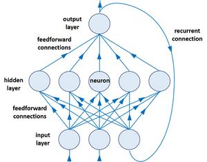
Feedforward networks are not well suited for analyzing sequential phenomena where the data at each time step is dependent on the previous time step. Recurring networks, networks with internal memory, have therefore been developed for the analysis of time series data. It usually has a single layer of hidden neurons. The output from each time step is buffered and fed back to this layer so that the next input is processed using the memory from previous steps (Fig. 3).
Convolution network
A convolution network is a neural network that contains a subset of neurons sharing the same weights and who's combined receptive fields cover an entire input. This network architecture enables the identification of patterns irrespective of their location in the dataset. Convolution neural networks are particularly suited for the recognition of special features in an image.
Bayesian neural network
Bayesian neural networks are networks with stochastic weights and biases. Bayesian inference is the learning process of finding (inferring) the full probability distribution over all weight parameters in the weight parameter space, the so-called posterior distribution. A Bayesian Neural Network (BNN) is the application of posterior inference for each weight (and bias) in a neural network architecture. This contrasts to the learning process for feedforward networks, i.e. trying to find the optimal weights using optimization through gradient descent. Determining the posterior weight distribution is at the core of Bayesian networks. This can only be done in an approximate way, by using techniques that try to mimic the posterior using a simpler, tractable family of distributions with sampling methods such as Markov Chain Monte Carlo (MCMC), or variational inference. Explanations can be found, for example, in Jospin et al. 2020[7]. Bayesian networks have several advantages over regular feedforward networks: they are data efficient by avoiding overfitting and they provide estimates of uncertainty in deep learning, with distinction between statistical ('aleatoric') uncertainty and so-called epistemic uncertainty related to model imperfection.
Genetic neural network
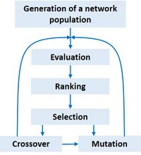
Genetic neural networks are inspired by genetics and use an analogous vocabulary with terms such as chromosomes, parents, breeding, reproduction, mutation, crossing, offspring and survival of the fittest. Genetic networks are often used in conjunction with standard feedforward networks. They circumvent some of the problems of these networks: the initial network design, slow gradient descent, and getting stuck in a local minimum. The genetic network algorithm starts by randomly creating a large population of neural networks and selecting from this population the specimens that perform best on a number of test data sets. Different performance criteria can be used, not only the best match with the test data, but also, for example, the simplicity of the network to avoid overfitting. From the selected specimens, a new generation of networks is created by randomly exchanging neurons or weights ('crossover') and introducing random mutations (Fig. 4). To perform these operations, the network specifications are encoded in binary strings ("chromosomes"). In a subsequent round of selection, the new best performing networks are selected and in turn used to create the next generation, and so on, until reaching a network with satisfactory performance. Diversity of the population is important for convergence to an optimal solution. The genetic algorithm does not use backpropagation and thus avoids some problems related to gradient descent by exploring a much wider range of network architectures and a very wide domain of the weight parameter space. However, the final convergence to an optimal solution is slow. Therefore, genetic neural networks are often used in combination with standard feedforward networks by creating an initial architecture and set of weight parameters that are already close to the optimum.
An accessible introduction to neural network methodologies is 'Deep learning' by J.D. Kelleher 2019[8]. A more advanced review of neural network methodologies is 'Deep learning' by LeCun et al. 2015[9].
Although models for artificial neural networks were originally developed to understand the dynamics of brain cells, there are now many applications that use artificial neural networks to analyze other types of data. Artificial neural networks have been applied to various aspects of coastal processes. When neural networks are used as a prediction tool, a crucial condition is that data used for training the network is not used for testing and prediction. The dataset must therefore always be split into parts.
Coastal applications of ANN
Artificial neural networks are currently used for analysis and prediction of various coastal processes[10]related to, for example, suspended sediment concentrations[11][12], seabed ripples[13][14], sandbank dynamics[15], beach planform [16], coastal erosion[17], salt marsh sedimentation[18], wave forecasting[19] and tidal forecasting[20]). A few typical examples are discussed below.
Littoral drift
Van Maanen et al (2010)[21] developed an artificial feedforward neural network (ANN) with backpropagation algorithm to predict the depth-integrated alongshore suspended sediment transport rate using 4 input variables (water depth, wave height and period, and alongshore velocity). The ANN was trained and validated using a dataset obtained from the intertidal beach of Egmond aan Zee, the Netherlands. 1522 data were used for training and 784 observations for validation. The best result was selected from 10,000 ANNs with different initial random weights. The ANN was shown to outperform the commonly used Bailard formula for littoral drift[22], even when this formula was calibrated. The alongshore component of the velocity, by itself or in combination with other input variables, had the largest explanatory power.
Nearshore sandbars
Pape and Ruessink (2011)[23] used linear and nonlinear recurrent networks to study the cross-shore motion of the outer longshore sandbar as a function of wave height. The recurrent network architecture is displayed schematically in Fig. 3. Two study sites with long-term observations were selected, the Gold Coast (GC, Australia) and Hasaki Oceanographic Research Station (HORS, Japan). The datasets covered 5600 daily-observed cross-shore sandbar locations and daily-averaged wave forcings. The time-series of sandbar data were divided into partitions of observed sandbar presence, some partitions being used for training and others prediction. Five different random initializations of the neural network weights for each training dataset resulted in slightly different optimal values of the weights, thus providing an estimate of the network accuracy. The results showed that many aspects of sandbar behavior, such as rapid offshore migration during storms, slower onshore return during quiet periods, seasonal cycles and annual to interannual onshore-directed trends can be predicted from the wave height with data-driven neural network models. Predictions were more accurate for offshore sandbar migration during high energy conditions than for onshore migration during periods of low waves, suggesting that onshore migration is less strongly correlated with wave height. The results also showed that sandbar migration correlates with wave height over a time scale of several days and not a single day. The linear and nonlinear networks had similar skill, the former performed better for HORS and the latter better for GC.
Beach nourishment
Bujak et al. (2021)[24] trained an ANN on shoreline evolution data of 68 beaches on the Croatian coast in order to predict beach nourishment requirements for 92 other Croatian beaches. The predictions were tested against field observations for these other beaches. To circumvent the issue of convergence to spurious local minima in the optimization process, 10 thousand ANNs were created with random initial weights. The tests revealed a strong correlation (coefficient 0.87) between the observations and the ANN’s output. The results showed that fetch length was the most important input variable for ANN’s prediction ability, apart from the basic information derived from maps such as beach length, beach area and beach orientation.
Extreme sea levels
Bruneau et al. (2020) [25] used the Global Extreme Sea Level Analysis database of quasi-global coastal sea level water information (from around 1070 tide gauges) and an ensemble of hourly physical predictors (wind, wave height and period, precipitation, ..) extracted from the high-resolution atmospheric reanalysis ERA5 of ECMWF[26] to estimate global sea level extremes using neural networks. Each gauge was modelled independently using artificial neural networks (ANNs), each composed of 3 hidden layers of 48 neurons. The input layer had 33 nodes (one for each environmental predictor combined with 7 hourly time steps of the harmonic tide), and the outer layer had a single node providing the non-tidal residual target. The ANN had just under 7000 trainable parameters. An ensemble of 20 ANNs was trained at each gauge location to generate a probabilistic forecast. Each ANN was fitted using 50% of the training set, randomly sampled. Because the test sets covered only one year at each gauge the most extreme skew surges were almost always underestimated compared to observations, but the neural network ensemble showed some skill in capturing them (over 2/3 of the signal) and systematically outperformed the multivariate linear regression.
Related articles
Data analysis techniques for the coastal zone
References
- ↑ Hodgkin, A. L. and Huxley, A. F. 1952. A quantitative description of ion currents and its applications to conduction and excitation in nerve membranes. J. Physiol. (London) 117: 500-544
- ↑ Gerstner, W. and Kistler, W.M. 2002. Spiking Neuron Models. Single Neurons, Populations, Plasticity. Cambridge University Press
- ↑ Rosenblatt, F. 1961. Principles of Neurodynamics, Spartan Press, Washington D.C.
- ↑ Kingston, K.S. 2003. Applications of Complex Adaptive Systems Approaches to Coastal Systems, PhD Thesis, University of Plymouth
- ↑ McCulloch, W.S. and Pitts, W.H. 1943. A Logical Calculus of Ideas Immanent in Nervous Activity. Bulletin of Mathematical Biophysics 5: 115-133
- ↑ Srivastava, N., Hinton, G., Krizhevsky, A., Sutskever, I. and Salakhutdinov, R. 2014. Dropout: a simple way to prevent neural networks from overfitting. J. Machine Learning Res. 15: 1929–1958
- ↑ Jospin, L.V., Laga, H., Boussaid, F., Buntine, W. and Bennamoin, M. 2007. Hands-on Bayesian Neural Networks – a Tutorial for Deep Learning Users. arXiv:2007.06823
- ↑ Kelleher, J.D. 2019. Deep learning. The MIT Press, Cambridge, Massachusetts.
- ↑ LeCun, Y., Bengio, Y. and Hinton, G. 2015. Deep learning. Nature 521(7553): 436-444
- ↑ Goldstein, E.B., Coco, G. and Plant, N.G. 2019. A review of machine learning applications to coastal sediment transport and morphodynamics. Earth-Science Reviews 194: 97-108
- ↑ Oehler, F., Coco, G., Green, M.O. and Bryan, K.R. 2011. A data-driven approach to predict 1073 suspended-sediment reference concentration under non-breaking waves. Continental Shelf Research 46: 96-106
- ↑ Yoon, H-D., Cox, D.T. and Kim, M. 2013. Prediction of time-dependent sediment suspension in the surf zone using artificial neural network. Coastal Engineering 71:78–86
- ↑ Yan, B., Zhang, Q. and Wai, O.W.H. 2008. Prediction of sand ripple geometry under waves using an artificial neural network. Computers & Geoscience 34: 1655-1664
- ↑ Goldstein, E. B., Coco, G. and Murray, A.B. 2013. Prediction of Wave Ripple Characteristics using Genetic Programming. Continental Shelf Research 71, 1-15
- ↑ Pape, L., Ruessink, B. G., Wiering, M. A. and Turner, I. L. 2007. Recurrent neural network modeling of nearshore sandbar behavior. Neural Networks 20: 509–518
- ↑ Iglesias, G., Lopez, I., Carballo, R. and Castro, A. 2009. Headland-bay beach planform and tidal range: a neural network model. Geomorphology 112: 135–143
- ↑ Tsekouras, G. E., Rigos, A., Chatzipavlis, A. and Velegrakis, A. 2015. A neural-fuzzy network based on Hermite polynomials to predict the coastal erosion. In Engineering Applications of Neural Networks (pp. 195-205). Springer International Publishing
- ↑ Coco, G., Ganthy, F., Sottolichio, A. and Verney, R. 2011. The use of Artificial Neural Networks to predict intertidal sedimentation and unravel vegetation effects. Proceedings of the 7th IAHR Symposium on River, Coastal, and Estuarine Morphodynamics, Beijing, China
- ↑ Deo, M.C. and Sridar Naidu, C. 1999. Real Time Wave Forecasting using Neural Networks. Ocean Engineering 26: 191-203
- ↑ Tsai, C.-P. and Lee T.-L. 1999. Back-Propagation Neural Network in Tidal-Level Forecasting. Journal of Waterway, Port, Coastal and Ocean Engineering 125: 195-202
- ↑ van Maanen, B., Coco, G., Bryan, K.R. and Ruessink, B.G. 2010. The use of artificial neural networks to analyze and predict alongshore sediment transport. Nonlinear Processes in Geophysics: 17: 395-404
- ↑ Bailard, J. A. 1981. An energetics total load sediment transport model for a plane sloping beach. J. Geophys. Res., 86: 10938–10954
- ↑ Pape, L. and Ruessink, G.B. 2011. Neural-network predictability experiments for nearshore sandbar migration. Continental Shelf Research 31: 1033-1042
- ↑ Bujak, D., Bogovac, T., Carevic, D., Ilic, S. and Loncar, G. 2021. Application of Artificial Neural Networks to Predict Beach Nourishment Volume Requirements. J. Mar. Sci. 9, 786
- ↑ Bruneau, N., Polton, J., Williams, J. and Holt, J. 2020. Estimation of global coastal sea level extremes using neural networks. Environ. Res. Lett. 15, 074030
Please note that others may also have edited the contents of this article.
|


