Stability models
Contents
Stability: concepts.
The concepts of equilibrium and stability come from Classical Mechanics. A state where a system is in balance with the external forcing so that it does not change in time is called an equilibrium position. However, any equilibrium position may be either stable or unstable. If released near a stable equilibrium position, the system will evolve towards such a position. On the contrary, if released near an unstable equilibrium position, it will go far away from this position. For instance, a pendulum has two equilibrium positions, one up (A), another down (B). If released at rest at any position (except at A) the pendulum will start to oscillate (if it is not already in B) and due to friction it will end up at rest at B. Thus, the pendulum will move spontaneously towards the stable equilibrium and far away from the unstable equilibrium.
Similarly, a beach under constant wave forcing is commonly assumed to reach after some time certain equilibrium profile. However, two main assumptions are here involved: i) an equilibrium state exists and ii) the equilibrium is stable. The existence of an equilibrium profile seems to be granted in the books on coastal sciences and the stability of such an equilibrium is implicitly assumed. However, even if an equilibrium profile exists, it is not necessarily stable. This means that the system would ignore such an equilibrium, it would never tend spontaneously to it. Furthermore, several equilibria may exist, some of them stable, some others unstable.
Example:
Let us assume a system which is described by only one variable as a function of time, [math]x(t)[/math], and two constant parameters [math] \alpha [/math] and [math] x_c \gt 0 [/math] which are representative of both the characteristics of the system and the external forcing. Assume that this variable is governed by the ordinary differential equation:
[math] \frac{dx}{dt} = \alpha (x-x_c)x [/math]
For instance, in a coastal system, [math] \alpha [/math] could represent sediment grain size or wave height, and [math]x(t)[/math] the shoreline displacement at an alongshore location. Given an initial position [math] x(0)=x_0 [/math], the subsequent evolution of the system is described by the solution of the differential equation
[math] x(t) = \frac{x_0 x_c}{x_0 +(x_c-x_0)exp(x_c \alpha t)}[/math]
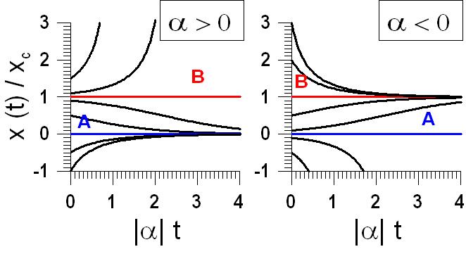
It becomes clear that the system has two equilibrium positions, (A): [math]x=0[/math], and (B): [math]x=x_c[/math]. Moreover, for [math] \alpha \gt 0[/math], (A) is stable while (B) is unstable. In contrast, (A) is unstble and (B) is stable for [math] \alpha \lt 0 [/math]. This is ilustrated by Fig. 1 where typical [math]x(t)[/math] solutions are plotted for various initial conditions.
 Fig.1: For [math]\alpha \gt 0[/math] (left) all the solutions starting in a neighborhood of [math]x=0[/math] tend to [math]x=0[/math] for [math]t \to \infty[/math] while there are solutions starting arbitrarily near [math]x=x_c[/math] that do not tend to [math]x=x_c[/math].