File list
This special page shows all uploaded files.
| Date | Name | Thumbnail | Size | User | Description | Versions |
|---|---|---|---|---|---|---|
| 10:07, 11 October 2016 | VanRijnFig7.jpg (file) |  |
67 KB | Dronkers J | Suspended transport as function of depth-averaged velocity. | 1 |
| 10:05, 11 October 2016 | VanRijnFig6.jpg (file) |  |
89 KB | Dronkers J | Time lag of suspended sediment concentration in tidal flow. | 1 |
| 10:03, 11 October 2016 | VanRijnFig5.jpg (file) |  |
46 KB | Dronkers J | Definition sketch of suspended sediment transport. | 1 |
| 10:02, 11 October 2016 | VanRijnFig3.jpg (file) |  |
99 KB | Dronkers J | Depth-averaged velocity at initiation of motion and suspension. | 1 |
| 10:01, 11 October 2016 | VanRijnFig2.jpg (file) |  |
64 KB | Dronkers J | Initiation of motion and suspension as function of dimensionless sediment size. | 1 |
| 10:00, 11 October 2016 | VanRijnFig1.jpg (file) |  |
144 KB | Dronkers J | Initiation of motion as function of Reynolds number. | 1 |
| 10:21, 10 October 2016 | VanRijnFig4.jpg (file) |  |
337 KB | Dronkers J | Bed forms in steady flows (rivers). | 1 |
| 16:57, 26 September 2016 | BaZaFig7.jpg (file) |  |
151 KB | Dronkers J | Example of integrated risk map, scale from 1 to 4 (from low to very high impact). | 1 |
| 16:55, 26 September 2016 | BaZaFig6.jpg (file) |  |
163 KB | Dronkers J | Example map of flooding velocities derived from the modified watershed segmentation algorithm. | 1 |
| 16:50, 26 September 2016 | BaZaFig5.jpg (file) |  |
74 KB | Dronkers J | Editing a mitigation option in front of Cesenatico. | 1 |
| 16:49, 26 September 2016 | BaZaFig4.jpg (file) |  |
85 KB | Dronkers J | Mitigation screen. | 1 |
| 16:49, 26 September 2016 | BaZaFig3.jpg (file) |  |
100 KB | Dronkers J | Scenarios screen. | 1 |
| 16:48, 26 September 2016 | BaZaFig2.jpg (file) |  |
121 KB | Dronkers J | The viewer at the start-up. | 1 |
| 16:47, 26 September 2016 | BaZaFig1.jpg (file) |  |
334 KB | Dronkers J | Key elements and the flow of information within THESEUS DSS. | 1 |
| 16:46, 26 September 2016 | BaZaTable1.jpg (file) |  |
241 KB | Dronkers J | Review of existing exploratory tools that can be used for supporting decisions applied to coastal areas. These GIS-based tools perform scenario construction and analysis. | 1 |
| 09:06, 19 September 2016 | LucianaFig.jpg (file) |  |
1.64 MB | Dronkers J | Geotextile tube application at the beach of Ofir, Esposende, Portugal. | 1 |
| 09:57, 15 September 2016 | GiovanniFig3.jpg (file) |  |
27 KB | Dronkers J | Figure 3. Beach cusp spacing as a function of swash excursion for measurements and numerical simulations. | 1 |
| 09:56, 15 September 2016 | GiovanniFig2.jpg (file) |  |
40 KB | Dronkers J | Figure 2. Flow circulation over beach cusps. | 1 |
| 09:37, 15 September 2016 | GiovanniFig4.jpg (file) |  |
23 KB | Dronkers J | Figure 4. Measured beach cusp spacing versus the spacing predicted assuming the presence of subharmonic (left panel) or synchronous (right panel) standing edge waves. | 1 |
| 15:35, 14 September 2016 | CocoFig4.jpg (file) |  |
20 KB | Dronkers J | Figure 4: Measured beach cusp spacing versus the spacing predicted assuming the presence of subharmonic standing edge waves. | 1 |
| 15:35, 14 September 2016 | CocoFig3.jpg (file) |  |
31 KB | Dronkers J | Figure 3: Beach cusp spacing as a function of swash excursion for measurements (field and laboratory) and numerical simulations. | 1 |
| 15:34, 14 September 2016 | Fig2.jpg (file) |  |
40 KB | Dronkers J | Figure 2: Snapshots of flow circulation over beach cusps. | 1 |
| 15:33, 14 September 2016 | CocoFig1.jpg (file) |  |
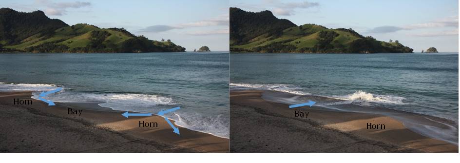
101 KB | Dronkers J | Figure 1: Beach cusps | 1 |
| 15:27, 13 September 2016 | LucianaTable1.jpg (file) |  |
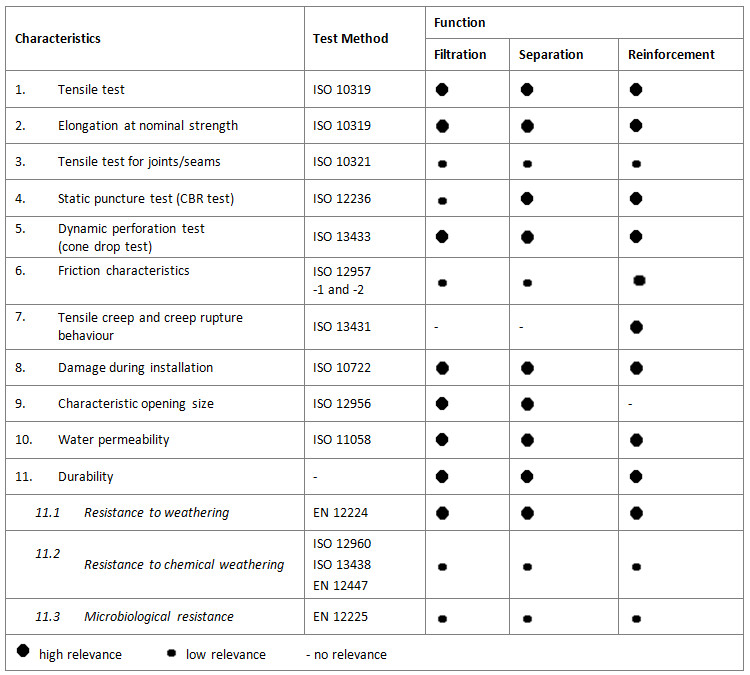
122 KB | Dronkers J | Table 1: Characteristics of geotextiles and geotextile-related products according to functions and test methods. | 1 |
| 15:26, 13 September 2016 | LucianaFig1.jpg (file) |  |
124 KB | Dronkers J | Fig 1. Iterative design process for sand-filled geosystems | 1 |
| 16:01, 31 August 2016 | Wapenschild Wenduine.jpg (file) |  |
20 KB | Stephies | 1 | |
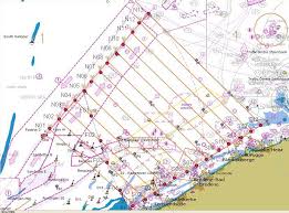
| 15:15, 31 August 2016 | Aerial line transects.jpg (file) | 12 KB | Stephies | 1 | ||
| 14:56, 31 August 2016 | Line transect BPNS.jpg (file) | 11 KB | Stephies | 1 | ||
| 12:50, 31 August 2016 | Skeleton harbour porpoise.jpg (file) |  |
64 KB | Stephies | 1 | |
| 11:43, 30 August 2016 | Figuur 6 installation wind turbines.jpg (file) |  |
154 KB | Stephies | 1 | |
| 11:26, 30 August 2016 | Figuur 9 hydrophones.gif (file) |  |
6 KB | Stephies | 1 | |
| 11:21, 30 August 2016 | Figuur 8 T-POD.jpg (file) |  |
149 KB | Stephies | 1 | |
| 11:10, 30 August 2016 | Figuur 3 Echolocation signals.gif (file) |  |
8 KB | Stephies | 1 | |
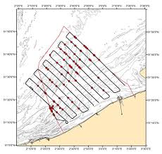
| 10:56, 30 August 2016 | Figuur 5 survey blocks.jpg (file) |  |
49 KB | Stephies | 1 | |
| 10:14, 30 August 2016 | Figuur 1 harbour porpoise.jpg (file) |  |
51 KB | Stephies | 1 | |
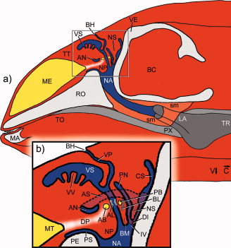
| 10:11, 30 August 2016 | Figuur 2 nasal complex.jpg (file) |  |
46 KB | Stephies | 2 | |
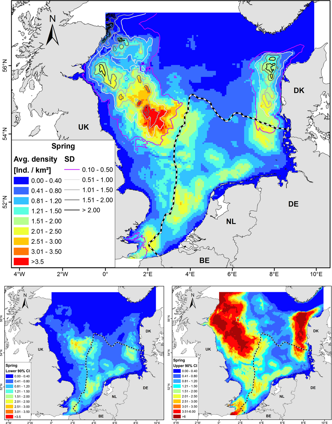
| 09:45, 30 August 2016 | Figuur 4 Predicted harbour porpoise density.png (file) |  |
917 KB | Stephies | 1 | |
| 13:50, 26 August 2016 | Figure fishing areas.jpeg (file) |  |
195 KB | Jozefiend | 1 | |
| 13:49, 26 August 2016 | Figure species.jpeg (file) |  |
65 KB | Jozefiend | 1 | |
| 10:46, 26 August 2016 | Grafiek soorten.jpeg (file) |  |
65 KB | Jozefiend | 1 | |
| 10:46, 26 August 2016 | Grafiek visgebieden.jpeg (file) |  |
195 KB | Jozefiend | 1 | |
| 17:56, 18 August 2016 | NienhuisFig3.jpg (file) |  |
33 KB | Dronkers J | Figure 3: Three deltas with varying wave influence. | 1 |
| 17:49, 18 August 2016 | NienhuisFig2.jpg (file) |  |
357 KB | Dronkers J | Figure 2: The Rio Grijalva in Mexico. | 1 |
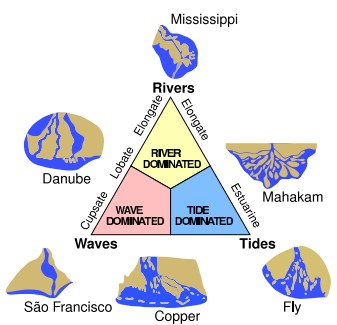
| 17:48, 18 August 2016 | NienhuisFig1.jpg (file) |  |
29 KB | Dronkers J | Figure 1: The ternary diagram of delta morphology. | 1 |
| 12:46, 13 August 2016 | Turkey.gif (file) |  |
37 KB | Pat Doody | 1 | |
| 11:53, 13 August 2016 | Romania.gif (file) |  |
10 KB | Pat Doody | 1 | |
| 22:44, 5 August 2016 | PrandleFig14.jpg (file) |  |
67 KB | Dronkers J | Figure 14. Tidal current amplitude, U, as a function of depth, D and tidal elevation amplitude, Z, based on bed friction coefficient, f= 0.0025. | 1 |
| 22:43, 5 August 2016 | PrandleFig13.jpg (file) |  |
40 KB | Dronkers J | Figure 13. ‘Equilibrium’ values of sediment concentrations and fall velocities. | 1 |
| 22:42, 5 August 2016 | PrandleFig12.jpg (file) |  |
123 KB | Dronkers J | Figure 12. Spring-neap variability in import vs export of sediments. | 1 |
| 22:41, 5 August 2016 | PrandleFig11.jpg (file) |  |
41 KB | Dronkers J | Figure 11. Schematic of dynamical and sedimentary components integrated into the analytical emulator. | 1 |